Finite Impulse Response Filters Using Apple's Accelerate Framework - Part III
In Part I and Part II of this series we developed a finite impulse response audio filter taking advantage of some of the DSP functions in the Accelerate Framework. The improvements we made in Part II were fairly straightforward, mostly replacing naive hand-coded loops with optimized implementations, taking advantage of specialized processor instructions to speed up our filter. In this installment, I’ll show you a less obvious improvement which can result in huge speedups for higher-order filters.
Instead of looking through our code for more opportunities to use vectorized code, in this part we’re going to turn to our DSP textbook (Oppenheim and Schaefer in my case, but any good text will cover this.) This last part of this series, we are going to take a different approach to convolution based on the convolution theorem.
The Convolution Theorem
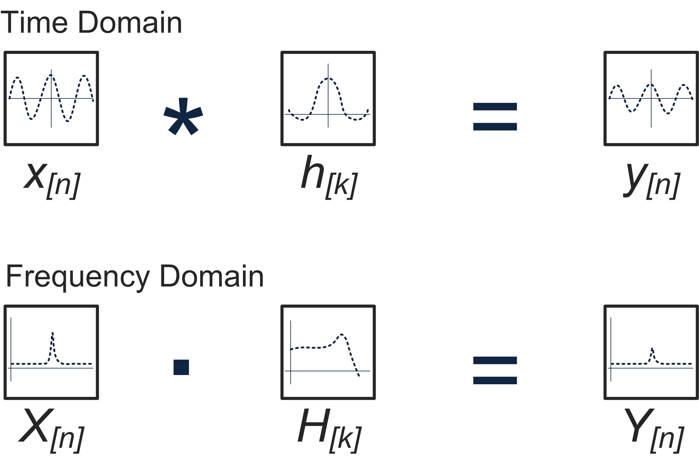
The convolution theorem states that convolution of two signals in the time domain is equivalent to the multiplication of their corresponding Fourier transforms. Essentially, we will obtain the same result if we multiply the Fourier transforms of our signals as we would if we convolved the signals directly.

The above image shows the convolution operation in both the time and frequency domains.
Applying The Convolution Theorem
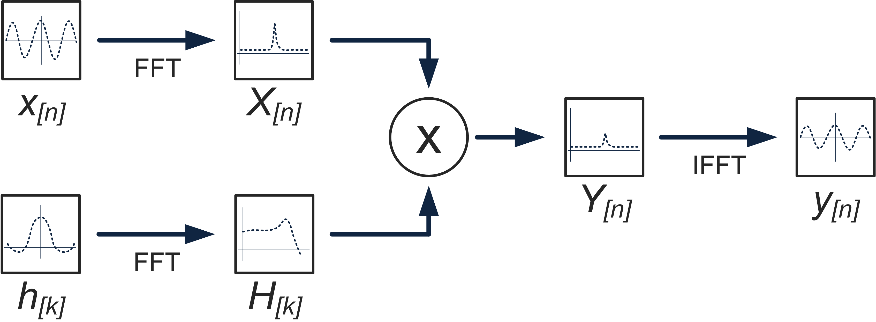
If you recall from an earlier post, our naive convolution function contained a set of nested loops which looped over the entire input signal and the entire filter kernel, multiplying each input sample with each filter tap and adding them up. According to the convolution theorem, if we have the frequency-domain representation of our signal and our filter, all we have to do is multiply them, which exponentially decreases the number of operations required to compute the convolution. In order to implement this topology, we need to compute the Discrete-time Fourier transform (DFT) of our input signal and our filter kernel, multiply the resulting frequency-domain signals, and then compute the inverse DFT to get our filtered signal. Naturally, we will use the Fast Fourier Transform (FFT) algorithm to compute the Fourier transforms. Our FFT-based convolution approach is shown in this block diagram:

FFT-convolution isn’t exactly a silver bullet, because even though we’ve drastically decreased the number of multiply-add cycles, we’ve added the overhead of computing the Fourier Transform of the input signal and filter, and computing the inverse Fourier transform of the result. For this reason, you should only use this approach to computing convolution when you have a long filter kernel. Conventional wisdom is to use FFT convolution for filter lengths longer than 64-128 samples, and to compute convolution directly otherwise. This is by no means a hard and fast rule, and the optimal cutoff point will vary based on a number of factors. As always, profile first!
Implementation Considerations
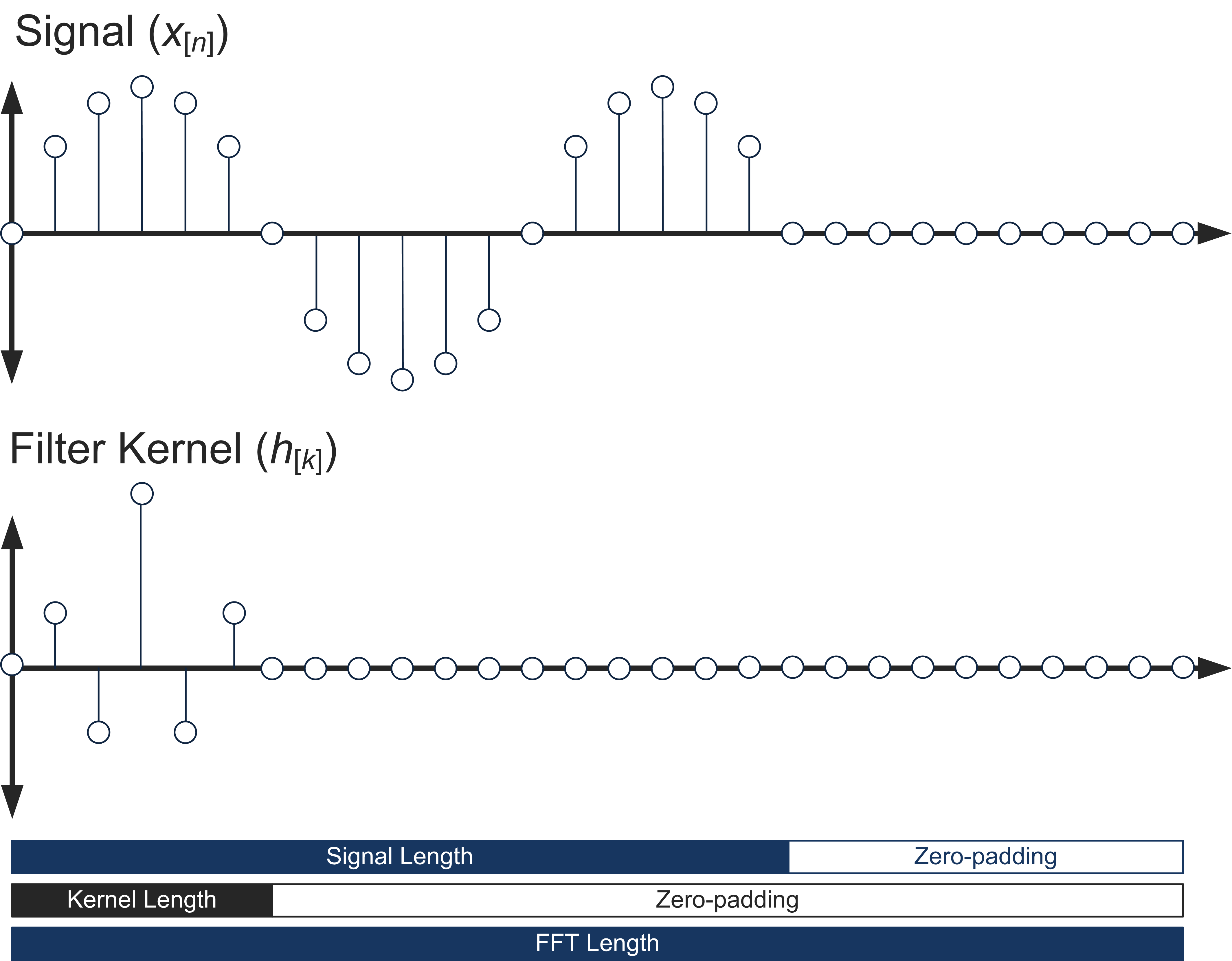
The first step in our convolution approach is to compute the DFTs of our input signal and our filter kernel. There are several things to consider at this point. Most importantly, the FFT algorithm is optimized for calculating the DFT of signals with a length that is a power of 2. Secondly, the lengths of the DFTs must be the same for both the signal and the filter kernel. We need to select our FFT length to be longer than our convolution length (signal length + kernel length – 1) as well as satisfying the power-of-2 requirement. We will choose the FFT length to be the next power of 2 greater than our convolution length. The way we change the length of our signal and our filter kernel is by zero-padding, which means nothing more than adding zeros onto the end until we reach the desired length. This is shown below:

Once we have selected our FFT length and zero-padded our signals, we can go ahead and compute the FFTs of our filter and input. If you know that your filter kernel is not changing, compute the FFT once at initialization and store it, to eliminate redundant calculation.
The multiplication and inverse DFT (IDFT) are straightforward, which leaves only the overlap-and-add method for handling the extra samples at the end of our filtered signal. This is handled in the same way as previously. The extra samples added when the zero-padding the signal and filter out to the next power-of-2 length will come out as zeros, we could process them as part of the overlap, adding them to the beginning of the next block, but they may be safely ignored.
The Implementation
#include <math.>
#include <Accelerate/Accelerate.h>

/* filter signal x with filter h and store the result in output.
 * output must be at least as long as x
 */

void
fft_fir_filter( const float *x,
                unsigned x_length,
                const float *h,
                unsigned h_length,
                float *output)
{

    // The length of the result from linear convolution is one less than the
    // sum of the lengths of the two inputs.
    unsigned result_length = x_length + h_length - 1;
    unsigned overlap_length = result_length - x_length;


    // Create buffer to store overflow across calls.
    //
    // This assumes that h_length doesn't change across calls.
    // The overflow buffer would usually be passed in rather
    // than being a static.
    static float *overflow = NULL;
    if (!overflow) {
        overflow = malloc(sizeof(float) * (h_length - 1));
        float zero = 0.0;
        vDSP_vfill(&zero, overflow, 1, h_length - 1);
    }

    // You need to implement next_pow2, it should return the first power of 2
    // greater than the argument passed to it.
    unsigned fft_length = next_pow2(result_length);


    // Create buffers to hold the zero-padded signal, filter kernel, and result.
    float h_padded[fft_length];
    float x_padded[fft_length];
    float temp_result[fft_length];

    // fill padded buffers with zeros
    float zero = 0.0;
    vDSP_vfill(&zero, h_padded, 1, fft_length);
    vDSP_vfill(&zero, x_padded, 1, fft_length);

    // Copy inputs into padded buffers
    cblas_scopy(h_length, h, 1, h_padded, 1);
    cblas_scopy(x_length, x, 1, x_padded, 1);


    // The Accelerate FFT needs an initialized setup structure. This, like much
    // of the above setup routine should be done outside of this function. I am
    // putting it here for ease of demonstration. This only needs to happen once.
    //
    // A balancing call to vDSP_destroy_fftsetup() is needed to prevent a
    // memory leak.
    FFTSetup setup = vDSP_create_fftsetup(log2f((float)fft_length), FFT_RADIX2);

    // Create complex buffers for holding the Fourier Transforms of h and x
    // DSPSplitComplex holds pointers to two arrays of values, real, and imaginary.
    // Each array should hold at least fft_length/2 samples.
    DSPSplitComplex     h_DFT;
    DSPSplitComplex     x_DFT;

    // Create and assign the backing storage structures for each of these buffers.
    // In your actual implementation, these should be allocated elsewhere and
    // passed to this function along with the FFTSetup from above.
    float h_real[fft_length/2];
    float h_imag[fft_length/2];
    h_DFT.realp = h_real;
    h_DFT.imagp = h_imag;

    float x_real[fft_length/2];
    float x_imag[fft_length/2];
    x_DFT.realp = x_real;
    x_DFT.imagp = x_imag;


    // Here we calculate the FFT of the filter kernel. This should be done once
    // when you initialize your filter. As I mentioned previously, much of
    // this setup routine should be done outside of this function and saved.

    // Convert the real-valued filter kernel to split-complex form
    // and store it in our DFT array.
    vDSP_ctoz((DSPComplex*)h_padded, 2, &h_DFT, 1, (fft_length/2));

    // Do in-place FFT of filter kernel
    vDSP_fft_zrip(setup, &h_DFT, 1, log2f(fft_length), FFT_FORWARD);


    // Calculate FFT of input signal...

    // Convert the real-valued signal to split-complex form
    // and store it in our DFT array.
    vDSP_ctoz((DSPComplex*)x_padded, 2, &x_DFT, 1, (fft_length/2));

    // Do in-place FFT of the input signal
    vDSP_fft_zrip(setup, &x_DFT, 1, log2f(fft_length), FFT_FORWARD);


    // This gets a bit strange. The vDSP FFT stores the real value at nyquist in the
    // first element in the imaginary array. The first imaginary element is always
    // zero, so no information is lost by doing this. The only issue is that we are
    // going to use a complex vector multiply function from vDSP and it doesn't
    // handle this format very well. We calculate this multiplication ourselves and
    // add it into our result later.

    // We'll need this later
    float nyquist_multiplied = h_DFT.imagp[0] * x_DFT.imagp[0];

    // Set the values in the arrays to 0 so they don't affect the multiplication
    h_DFT.imagp[0] = 0.0;
    x_DFT.imagp[0] = 0.0;

    // Complex multiply x_DFT by h_DFT and store the result in x_DFT
    vDSP_zvmul(&x_DFT, 1, &h_DFT, 1, &x_DFT,1, fft_length/2, 1);

    // Now we put our hand-calculated nyquist value back
    x_DFT.imagp[0] = nyquist_multiplied;


    // Do the inverse FFT of our result
    vDSP_fft_zrip(setup, &x_DFT, 1, log2f(fft_length), FFT_INVERSE);

    // And convert split-complex format to real-valued
    vDSP_ztoc(&x_DFT, 1, (DSPComplex*)temp_result, 2, fft_length/2);

    // Now we have to scale our result by 1/(4*fft_length)
    // (This is Apple's convention) to get our correct result.
    float scale = (1.0 / (4.0 * fft_length) );
    vDSP_vsmul(temp_result, 1, &scale, temp_result, 1, fft_length);


    // The rest of our overlap handling is the same as in our previous
    // implementation

    // Add the overlap from the previous run
    // use vDSP_vadd instead of loop
    vDSP_vadd(temp_result, 1, overflow, 1, temp_result, 1, overlap_length);

    // Copy overlap into overlap buffer
    cblas_scopy(overlap_length, temp_result + x_length, 1, overflow, 1);

    // write the final result to the output. use BLAS copy instead of loop
    cblas_scopy(x_length, temp_result, 1, output, 1);
}
There are many improvements that need to be made to the above code, primarily moving redundant code outside of the processing loop and into an initialization routine. There are also many opportunities for refactoring. I personally use a thin abstraction layer over the FFT functions, which eliminates the need to re-write the conversions between split and interleaved complex types and things like that. For prototyping and general development, having functions like: FFT(input, output, length); and IFFT(input, output, length) save a lot of time. I will dive into the vDSP_fft functions in more depth for a future post.
Edit: Thanks to Ricci Adams for some corrections and additions!